 Algorithms Anonymous
- 38 mins CLRS Problem Set Solutions
Table of Contents
- Problem Set 01
- Problem Set 02
- Problem Set 03
- Problem Set 04
- Problem Set 05
- Problem Set 06
- Problem Set 07
This is a collection of course work, mostly consisting of problems taken from the CLRS MIT Press textbook. The algorithms course was completed in December of 2018. This repository is a demonstration of my own personal understanding of the material covered. There are a total of eleven problem sets in all. The first half deals mainly with a slightly more mathematically rigorous look into some classic data structures and algorithms. Then we’ll dive into a more exciting domain (graphs!) and explore more awesome concepts!
Note to reader: Problem sets are currently in the process of being transmogrified into this GitHub page.
Problem set 01
A collection of loop invariant proofs, as well as a recurrence tree proof. The algorithms involved in this problem set include:
- linear search
- binary search
- bubble sort
Linear Search
LinearSearch(A, n, v)
  for i = 0 to n - 1
    if A[i] == v
      return i
  return NIL
Loop invariant:
At the start of each iteration of the for loop, the sub-array A’[0..i - 1] does not contain the value v.
Initialization:
When the for loop is read, i = 0, thus the sub-array A’ is empty. Therefore the invariant is vacuously true.
Maintenance:
With each iteration, assume A’[0..i - 1] does not contain v, if A[ i ] == v, i is returned. Otherwise, i = i + 1. So, we have…
i - 1 = (i - 1) + 1
i - 1 = i
Therefore the invariant is maintained.
Termination:
if i = n - 1 and A[ i ] != v, then i = n and the loop exits. Because the invariant was maintained, the sub-array A’[0..i - 1] does not contain v, but i = n. So, we have…
i - 1 = n - 1
Therefore A[0..n - 1] does not contain v.
QED
Binary Search
BinarySearch(x, A, min, max)
  low = min
  high = max
  while low <= high
    mid = floor( (low + high) / 2 )
    if x < A[mid]
      high = mid - 1
    else if x > A[mid]
      high = mid + 1
    else
      return mid
  return NIL
A recurrence relation can be defined to represent binary search as follows…
T(n) = aT(n / b) + D(n) + C(n)
Assume T(1) = Θ(1) = c
Let D(n) be the cost to divide and C(n) be the cost to compare.
D(n) = ⌊(low + high) / 2⌋ = Θ(1) = c
Where low and high are the respective indices corresponding to the sub-arrays within each level of recursion.
It is easy to see C(n) = Θ(1), as only a single key comparison occurs in the array Ak on the kth call to T(n).
For the values of a and b, binary search divides the problem in half, working on only one of the resulting halves. This gives us…
a = 1 and b = 2
So, putting this all together we have…
T(n) = T(n / 2) + Θ(1) + Θ(1)
= T(n / 2) + Θ(1)
= T(n / 2) + c
Where c = T(1)
If defined as a recurrence tree, binary search could be thought of as a path from the root to a single leaf, as only one edge per level is traversed.
Or, c + c + … + c
= c(1 + 1 + … + 1)
Claim: c(1 + 1 + … + 1) = c(log2(n) + 1)
Proof:
Base case: n = 1
Hypothesis: The levels of a tree with 2i leaves = log2(2i) + 1 = i + 1
Let n = 2i + 1
log2(2i + 1) + 1 = i + 1 + 1
(i + 1)log22 + 1 = i + 2
i + 2 = i + 2
Therefore in the worst case, binary search has a constant cost, c, log2(n) + 1 times, or…
c(log2(n) + 1)
= clog2(n) + c
= Θ(log2(n))
QED
Bubble Sort
One of the main benefits of bubble sort is early termination if no ‘bubbling’ occurs. In this example, no such consideration is taken.
BubbleSort(A)
  for i = 1 to A.length - 1
    for j = A.length downto i + 1
      if A[j] < A[j - 1]
        exchange A[j] with A[j - 1]
This implementation also takes a ‘bubble down’ approach. Our proof will attack the inner loop first, working our way out.
Loop Invariant:
At the start of each iteration of the inner loop, the element A[ j ] ≤ A[ j + 1 ].
Initialization:
When the loop begins, j = A.length, because no element exists at A[ j + 1 ] the invariant is vacuously true.
Maintenance:
With each successive iteration, if A[ j ] < A[ j - 1 ] then the values are exchanged. Because j is decremented, j = j - 1. Therefore the exchange results in A[ j ] ≤ A[ j + 1 ] by susbstituting the values of j.
Termination:
When j = i + 1, the comparison taking place occurs between j and i because i = j - 1. When j is decremented once more, the loop exits with j = i. The invariant was maintained, thus by substitution…
A[ i ] ≤ A[ i + 1 ]
Let us now use this result to prove correctness of the outer loop…
Loop Invariant:
The Array A’ consists of the elements A[ 1..i ] such that A’[ 1 ] ≤ A’[ 2 ] ≤ … ≤ A’[ i ]
Initialization:
The loop begins with i = 1, thus the invariant vacuously holds for an array of size one.
Maintenance:
With each iteration of the outer loop, we showed that termination of the inner loop results in A[ i ] ≤ A[ i + 1 ]. Each pass then increments i, resulting in i = i + 1, but this means A[ i - 1 ] ≤ A[ i ]. Therefore A’ is maintained.
Termination:
When i = A.length the loop exits. Maintenance shows that A’[ 1 ] ≤ A’[ 2 ] ≤ … ≤ A’[ i ], but i = A.length. Therefor A’[1..A.length] is the output.
QED
Analysis:
In the worst case, the inner loop iterates n - (i + 1) + 1 or n - i times in relation to the outer loop.
So,
i = 1 : j = n - 1
i = 2 : j = n - 2
.
.
.
i = n - 1 : j = 1
Which is equivalent to…
(n - 1) + (n - 2) + (n - 3) + … + 1
= n(n - 1) / 2
= (n2 - n) / 2
= O(n2)
In our implementation we can make this a tight bound of Θ(n2) because no optimization takes place.
Problem Set 02
A collection of asymptotic proofs, in regard to defining a handful of functions into sets of O, Θ, Ω, as well as o, θ, ω. We will also take a brief look into binary trees, along with an analysis of a merge-insertion sort hybrid algorithm.
Asymptotic Analysis
| f(n) | g(n) | O | o | Ω | ω | Θ |
|---|---|---|---|---|---|---|
| 4n2 | 4lgn | 1 | 0 | 1 | 0 | 1 |
| 2lgn | lg2n | 0 | 0 | 1 | 1 | 0 |
| n1/2 | nsin n | 0 | 0 | 0 | 0 | 0 |
The following simple mathematical proofs will serve as confirmation for the above table. For every proof, we assume c and n ∈ R, and that each holds ∀n | n ≥ n0 with n0 ≥ 0.
Row 1
Big-O / Little-o
Let f(n) = 4n2 and g(n) = 4lgn
Assume f(n) = O( g(n) )
Then 0 ≤ f(n) ≤ cg(n)
4n2 ≤ c4lgn
≤ c(22)lgn
≤ c22lgn
≤ c2lgn2
≤ cn2
So,
0 ≤ 4n2 ≤ cn2
Let c = 4 and n0 = 1
∴ f(n) = O( g(n) )
We can easily show that little-o does not apply here as Big-O was proved by showing equality of f and g.
∴ f(n) ≠ o( g(n) )
Big-Omega / Little-omega
Assume f(n) = Ω( g(n) )
Then 0 ≤ cg(n) ≤ f(n)
We can easily show this by the equality shown in the Big-O proof.
∴ f(n) = Ω( g(n) )
Similarly to little-o, the equality of f and g proves f(n) ≠ ω( g(n) )
Big-Theta
Assume f(n) = Θ( g(n) )
Then 0 ≤ c1g(n) ≤ f(n) ≤ c2g(n)
Let c1 = c2 = 4 and n0 = 1
We have, 0 ≤ 4n2 ≤ 4n2 ≤ 4n2
∴ f(n) = Θ( g(n) )
QED
Row 2
Big-O / little-o
Let f(n) = 2lgn and g(n) = lg2n
Assume f(n) = O( g(n) )
Then 0 ≤ 2lgn ≤ clg2n
2lgn = n
lg( 2lgn ) = lg(n)
lg(n) * lg(2) = lg(n)
lg(n) = lg(n)
n = n
So we have,
0 ≤ n ≤ clg2n
But any linear function will grow faster than any logarithmic function given large enough values of n.
∴ f(n) ≠ O( g(n) )
If f(n) ≠ O( g(n) ) then it is certainly not o( g(n) ).
That is, f(n) ≥ cg(n) where c = 1 and ∀n : n ≥ 16
∴ f(n) ≠ o( g(n) )
Big-Omega / little-omega
Assume f(n) = Ω( g(n) )
Let c = 1 and n0 = 16
Then 0 ≤ lg2n ≤ n holds true ∀n ≥ 16
∴ f(n) = Ω( g(n) )
Big-Theta
Because f(n) ≠ O( g(n) ), f(n) cannot be tightly bounded by g(n).
∴ f(n) ≠ Θ( g(n) )
QED
Row 3
The functions, √n and nsin(n), are not asymptotically comparable because the exponent of the sinusoidal function nsin(n) oscillates between the values 1 and -1.
Print Binary Tree
Below is a non-recursive pre-order traversal of a binary tree, written in Java. The traversal prints each node using a stack as an auxiliary data structure. We assume the tree consists of objects of the class TreeNode. We also assume the toString method has been overridden to print that data from the node in a desirable format.
public class BinaryTree {

  // Assume TreeNode class, member variables and methods

  private void PrintBinaryTreeNodes(TreeNode root) {
    if (root == null) {
      return;
    }

    Stack<TreeNode> treeStack = new Stack<>();
    treeStack.push(root);

    while (!stack.isEmpty()) {
      TreeNode node = treeStack.pop();
      node.toString();

      if (node.right != null) {
        treeStack.push(node.right);
      }

      if (node.left != null) {
        treeStack.push(node.left);
      }
    }
  }
}
Analysis
The algorithm works in O(n) time. The while loop takes a TreeNode as the root and prints it. Each subsequent node is pushed on the stack. For a pre-order traversal, the left child is pushed after the right, given the first-in last-out nature of a stack. So, every right sub-tree is appended until all left sub-roots have been popped and printed. The stack then maintains the order of visitation within the tree. Thus, we have n nodes entering the stack, with each node being operated on in O(1) time.
∴ PrintBinaryTreeNodes operates in O(n) time.
Merge Insertion Sort
The idea for a hybridization of merge sort and insertion sort depends on the fact that, given a small enough list size, insertion sort outperforms merge sort. Insertion sort can also sort in-place, giving it an advantage when implemented on most machines. The idea then is to coarsen the leaves of the merge sort recursion tree by calling insertion sort when the list size becomes sufficiently small. We will show the time-complexity in two parts, then find a bound for values of k…
Claim:
Insertion sort can sort n / k sub-lists, each of length k, in Θ(nk)
Proof:
Let us take a set of n elements and split it into k subsets of length n / k.
We are then sorting a set of k elements n / k times, or…
In terms of a recursion tree, merge sort originally bottoms out when the length of the set is 1. Instead, we are now bottoming out when the set has a length of size n / k, or…
Thus, the height of the hybridized recursion tree is lg (n / k) + 1, with a cost of cn at each level.
So, T(n) = cn ( lg (n / k) + 1 )
= Θ( n lg (n / k) )
Putting these two results together, we have the total cost of our algorithm as the sum of the constituent parts…
Θ( nk + n lg (n / k) )
A bound on the value of k
It is easy to see that if k were larger than O(lgn) than the value of k would become more than a constant factor.
This can be shown by substituting the bound on k into our hybrid’s complexity equation, and as result, simplifying back to the original time-complexity for merge sort.
Let k = O( lgn ) = lgn
Θ( n lgn + n lg (n / lgn) )
n / lgn must certainly grow slower than n, thus the leading expression dominates.
This results in Θ( n lgn ).
QED
IRL
Constants pertaining to the particular instances of the algorithms, the languages they are written in, and the machines they will be running on all affect performance. As such, using our analytical findings in conjunction with performance testing would give us an optimal solution for k.
We could simply run a series of tests, setting the value of k to the upper bound we found through analysis. We then run the sort, decrementing the value of k with each test case. After which, we then analyze the data looking for the optimal value for the length of the sub-lists.
Problem Set 03
Expected Length of a Coding Scheme
This simple exercise will look at the expected bit-length of 3 character encoding schemes. The set of characters for all of these cases is: {A, B, C, D, E}. The first scheme uses a 3-bit encoding for all 5 characters, i.e.,
A => 001
B => 010
C => 011
D => 100
E => 101
The characters in our set occur with the following probabilities:
Pr[A] = 0.3 ; Pr[B] = 0.3 ; Pr[C] = 0.2 ; Pr[D] = 0.1 ; Pr[E] = 0.1
Let Xn be the expected length of encoding n letters
Then Xn = n (3Pr[A] + 3Pr[B] + 3Pr[C] + 3Pr[D] + 3Pr[E])
= n (3(0.3) + 3(0.3) + 3(0.2) + 3(0.1) + 3(0.1))
= 3n
We now evaluate using the same probability distribution, but a different encoding length:
A => 0
B => 10
C => 110
D => 1110
E => 1111
We will set up the following scheme:
A : 0 : A.length = 1 : Pr[A] = 0.3
B : 10 : B.length = 2 : Pr[B] = 0.3
C : 110 : C.length = 3 : Pr[C] = 0.2
D : 1110 : D.length = 4 : Pr[D] = 0.1
E : 1111 : E.length = 5 : Pr[E] = 0.1
Again we let Xn be the expected length of encoding n letters…
Xn = n (0.3 + 2(0.3) + 3(0.2) + 4(0.1) + 4(0.1))
= 2.3n
For the final encoding we use the same encoding length, but the probability distribution has changed to…
Pr[A] = 0.5 ; Pr[B] = 0.2 ; Pr[C] = 0.2 ; Pr[D] = 0.05 ; Pr[E] = 0.05
With this scheme we have the equation…
n (0.3 + 2(0.3) + 3(0.2) + 4(0.05) + 4(0.05))
= 1.9n
Hashing with Chaining
We now consider a hash table with m slots that uses chaining for collision resolution. With the table initially empty, we will find the probability that a chain of size k exists after k insertions.
Proof:
Xk = After k keys, there is a chain of size k
= I { k h( k ) = n } , where n is some slot in the table.
The probability of a key mapping to some slot is 1 / m. The following k - 1 keys must also map to the same slot.
∴ Xk = 1 / mk - 1
Working on a way to format hash tables in an aesthetically pleasing way, until then this section will be somewhat bare…
Skip Lists
(coming soon! Again with the aesthetics…)
Problem Set 04
In this problem set we will tackle a few recurrence relations using the Master Method. For one of those relations, we will use our findings from the MM to use as our guess within the substitution method. Where will see that sometimes less really is more!
After, we’ll take a deeper look into binary search trees. We will first prove a basic lemma by showing that the individual parts are true. Then we’ll run through an exercise in modifying a deletion algorithm. Finishing up with an algorithm to construct a balanced binary search tree along with a time complexity analysis.
Master Method
T(n) = 2 T( n / 4 ) + √n
a = 2 ; b = 4 ; f (n) = n1/2
But nlog42 = n1/2
So, in the relation we can express f as an element of the set Θ( nlogba ). By case 2 of the master theorem, this tells us that T(n) = Θ(√n * lgn).
QED
T(n) = 3 T( n / 9 ) + n3
a = 3 ; b = 9 ; f (n) = n3
nlog93 = n1/2
So, we have the cost at each level of the recurrence tree as an element of the set Ω( n1/2 + ε ) where ε = 5 / 2.
When using a lower bound on our cost function , we must perform a check according to the method:
a f ( n / b ) ≤ c f (n) for some c < 1 and sufficiently large values of n.
3 ( n / 9 )3 ≤ c f (n)
3 ( n / 32 )3 ≤
( 3n3 / 36 ) ≤
( n3 / 35 ) ≤ c n3
We can arbitrarily choose c = 1 / 3
∴ T(n) = Θ( n3 )
QED
T(n) = 7 T( n / 3 ) + n
a = 7 ; b = 3 ; f (n) = n
nlog37 > n
So, f (n) = O (nlog37 - ε) for some constant ε > 0
∴ T(n) = Θ( nlog37 ) by case 3 of the Master Theorem.
Substitution
Here, we will use the above result from the relation…
T(n) = 7 T( n / 3 ) + n
Guess: T(n) = Θ( nlog37 )
We must show that 0 ≤ cnlog37 ≤ T(n) ≤ cnlog37
0 ≤ c( n / 3 )log37 + n ≤ T(n) ≤ c( n / 3 )log37 + n
0 ≤ c( n )log37 + n ≤ T(n) ≤ c( n )log37 + n
This is where our attempt breaks down as there is no way to remove n from the inequality as to match our guess.
Let’s instead guess T(n) = Θ( nlog37 ) - dn
0 ≤ c( n )log37 + n - dn ≤ T(n) ≤ c( n )log37 + n - dn
Thus when d = 1 our inequality holds.
QED
More Fun with Binary Search Trees
Lemmas
The lemma to be proven:
If a node X in a binary search tree has two children, then its successor S has no left child and its predecessor P has no right child.
Claim:
The successor S cannot be an ancestor or cousin of X
Proof:
Suppose that the successor S is an ancestor or cousin of X.
S, the successor is an ancestor, but S must also reside in the minimum of X’s right subtree. Surely this is impossible! Consider now that S is a cousin of X, which means it resides at the same level with a different parent. However, this implies X and S and not separated by an intermediate node because S is X’s successor, but two nodes that are cousins are surely separated by a common ancestor above the parent!
∴ our hypothesis is a contradiction.
Claim:
if X has two children, the successor S must then be contained in it’s right sub tree such that the successor is the key with th minimum value.
Proof:
Suppose not, that is suppose X’s successor is not located at the minimum of X’s right subtree. There are only two other positions then: S is the parent of X, or S is somewhere in X’s left subtree.
Case 1: S is the parent of X. We know that X has two children. So then S would be a successor to multiple nodes, surely this contradicts the structure of a binary search tree.
Case 2: S is somewhere in X’s left subtree. If this were the case then S would both precede and succeed X, but this is impossible!
∴ our negated hypothesis is a contradiction.
Claim:
S cannot have a left child.
Proof:
Again, suppose not. That is, suppose S does have a left child. We showed before that S is the minimum of X’s right sub tree. If S has a left child that child is the minimum or else contains the minimum, but if S is the successor then it is also the minimum. This is impossible! There is only one minimum!
QED
Deletion
The pseudocode for Tree-Delete (pg.298 CLRS)
TREE-DELETE(T, z)
  if z.left == NIL
    Transplant(T, z, z.right)
  else if z.right == NIL
    Transplant(T, z, z.left)
  else
    y = Tree_Minimum(z.right)
    if y.p != Z
      Transplant(T, y, y.right)
      y.right = z.right
      y.right.p = y
    Transplant(T, z, y)
    y.left = z.left
    y.left.p = y
The above pseudocode relies on the logic of the above lemma when finding the successor node to replace the deleted node in the event that the right sub tree is not NULL.
The following is a modification of the foregoing code using the predecessor rather than the successor…
TREE-DELETE(T, z)
  if z.left == NIL
    Transplant(T, z, z.right)
  else if z.right == NIL
    Transplant(T, z, z.left)
  else
    y = Tree_Minimum(z.left)
    if y.p != Z
      Transplant(T, y, y.left)
      y.left = z.left
      y.left.p = y
    Transplant(T, z, y)
    y.right = z.right
    y.right.p = y
As one can easily see, the symmetry of the binary tree structure also us to take a ‘mirror image,’ so to speak.
Constructing Balanced Trees
Binary trees can become linear if special care is not taken in regard to how a particular implementation of the tree is built. We focus on balance here. That is, we recursively define a balanced binary tree with balanced binary sub trees. Here we assume a sorted array is passed as the actual parameter.
BalancedBinaryTree(A, start, end)
  if start > end
    return NIL

  middle = floor((start + end) / 2)
  node = A[middle]

  node.left = BalancedBinaryTree(A, start, middle - 1)
  node.right = BalancedBinaryTree(A, middle + 1, end)

  return node
The two recurrence calls in the above code split the problem in to two parts. Each subsequent problem is half the size of the array passed as the parameter. A constant cost at each level of recursion is required to compute the middle variable and assign pointers between nodes.
Thus we have T(n) = 2 T( n / 2 ) + c
The recursion is obviously dominated by the leaves…
c = O ( nlg 2 - ε ) where ε = 1
∴ T(n) = Θ(n) by case 1 of the Master Theorem
Problem Set 05
Things are picking up momentum and getting a bit more interesting in problem set 05. We’ll be taking an in-depth look into d-ary heaps. This will include diving into a height analysis, along with implementations of Extract_Max and Insert, with corresponding analyses for each.
We then pay a small homage to Dijkstra with an implementation of a 3_Way_Quicksort. A powerful approach in the respect that such an algorithm addresses the weakness Quicksort has when it comes to sorted, reverse sorted, or nearly sorted inputs.
D-Ary Heaps
To start things off, let’s take a look at how one would represent a d-ary heap in an array. We can accomplish this by verifying the following two formulas:
jth-child ( i, j ) = d ( i - 1 ) + j + 1
D_Ary_Parent ( i ) = floor ( ( i - 2 ) / d ) + 1
We will verify by way of a kind of inverse identity…
Claim:
D_Ary_Parent ( jth-child ( i, j ) ) = i
Proof:
Let us assume we are considering the first child so that j = 1
floor ( [ d ( i - 1 ) + 1 + 1 - 2 ] / d ) + 1 = i
= [ d ( i - 1 ) ] / d + 1
= i - 1 + 1
= i
QED
Height of a d-ary heap
The number of nodes in a completely filled i th level of some d-ary heap would of course be d i. Let us agree that the last filled level is the k th level. The number of nodes must then be the sum from level 0 to level k.
Or, d 0 + d 1 + d 2 + … + d k
Which is of course the simple geometric series…
The last node must reside in the filled level, or else it exists in the succeeding partially filled level, k + 1.
Our final node, let’s call it n, can be represented with the following inequality…
The inequality holds for k, but in the case of a partial level we would take the ceiling of the logarithm because at least k + 1 levels are needed as levels are discrete.
∴ The height of a d-ary heap of n elements is…
⌈ logd ( n ( d - 1 ) + 1 ) ⌉ - 1
Using the change of base formula this can be seen as…
Θ ( lg ( nd ) )
QED
Extract_Max
To implement extract max on a d-ary heap would remain the same as an implementation on a binary heap, except for an alteration to the Max_Heapify sub-routine. The code would be altered to simply find the largest element j, such that…
j = max ( A[ i ], the children of A[ i ] )
Therefore each node is compared to it’s d children
for j = 1 to d
  max = A[i]
  if A[j] > A[i]
    max = A[j]
return max
This results in Extract_Max’s run-time being Θ ( d lgn )
Insert
This particular implementation would also remain the same as a binary heap. That is, the key would be inserted at the last position of the heap, then the Heap_Increase_Key sub-routine would be called on the newly inserted key. If a key were greater than the parent, then it is also surely greater than it’s siblings. Thus the implementation does not change. The key is swapped with it’s corresponding parent until the correct position in the heap is found. In the worst case the new key belongs at the root.
∴ Insert = Θ ( h )
= Θ ( lg ( nd ) )
3 Way Quicksort
See also Dutch National Flag Problem
Here is a recursive implementation written in python…
def 3_Way_Partition(A, p, r):
  e, g, q = p, r, A[r]
  i = e

  while i < r:
    if A[i] < q:
      A[i], A[e] = A[e], A[i]
      e += 1
    elif A[i] > q:
      A[i], A[g] = A[g], A[i]
      g -= 1
      i -= 1
    i += 1
  return e, g

def 3_Way_Quicksort(A, p, r):
  if p < r:
    e, g = 3_Way_Partition
    3_Way_Quicksort(A, p, e - 1)
    3_Way_Quicksort(A, g + 1, r)
If we assume a balanced partitioning of 3_Way_Quicksort, we still have 2 sub-problems each half the size of the original. For random valued keys as the partition A[ e..g ] could be empty with a high probability.
Thus, T( n ) = 2 T ( n / 2 ) + Θ ( n )
= Θ ( n lgn ) by the Master Theorem
Now in the case of n identical items, 3_Way_Partition is adaptive as it will iterate over the n elements only one time. By doing this it creates a partition where p = e and g = r. In other words, the conditional base case of the recursion is true for a single call to 3_Way_Quicksort, namely the initial call.
T( n ) = 0 T ( n / 2 ) + Θ ( n )
= Θ ( n )
QED
Problem Set 06
We have past the half way point and find ourselves dealing with ways to escape the clutches of O(nlgn) comparison based sorting. After that, we work with red-black trees and they’re equivalent (2, 4) representations.
Sorting Large Numbers
What we are faced with is the task of sorting n integers in the range of 0 to n 4 - 1 in O( n ) time.
Let’s look at Counting_Sort as an option…
From CLRS (pg. 195)
Counting_Sort(A, b, k)
  let C[0..k] be a new array
  for i = 0 to k
    C[i] = 0
  for j = 1 to A.length
    C[A[j]] = C[A[j]] + 1
.
.
.
We need only examine the first for loop to see that Counting_Sort does not accomplish our goal. The loop iterates i = 0 to k, menaing Θ( k ) time. The overall time remains as Θ( n + k ), but k = n 4 - 1.
Thus the best run time that Counting_Sort can achieve is Θ( n 4 ). Which certainly does not achieve our goal of a linear sorting time.
Let’s instead take a look into Radix_Sort…
From CLRS (pg. 198)
Radix_Sort(A, d)
  for i = 1 to d
    use a stable sort to sort array A on digit i
Again, our problem consists of n integers ranging in values from 0 to n 4 - 1. Then we have d = logk( n ) digits. In the worst case d is not constant and thus with base-10 counting, k is in the domain [0, 9].
Radix_Sort = Θ ( logk( n )( n + 10) )
= Θ( n lgn )
We need to make a slight change to our representation of the integers comprising our array if we wish to achieve escape velocity, if you will, from the Θ( n lgn ) bound.
The issue with an unmodified Radix_Sort is the logarithmic term corresponding to the amount of digits to loop through. In the foregoing attempt we used base-10 digits, thus k = 10. and d = logk( n ). Instead, if we let k = n then our n integers are represented as base-n giving us…
Modified_Radix_Sort = Θ( logn( n )( n + n) )
= Θ( 2n)
= Θ( n )
Our goal has been achieved!
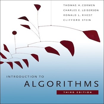
Red Black Trees
Everyone’s favorite! …Anyway, we are going to take an in-depth look into the CLRS code for deletion. We will first take a look at a deletion that results in a fairly ‘quick fix,’ then move on to a bit more complex scenario.
For each RB_Delete call we will state the property that is violated, as well as the case, in both the CLRS + Goodrich & Tamassia texts, that occurs at each state of the fix-up process.
We will be working with the following tree for each individual call to RB_Delete, i.e., the second call doesn’t work off the result of the first…
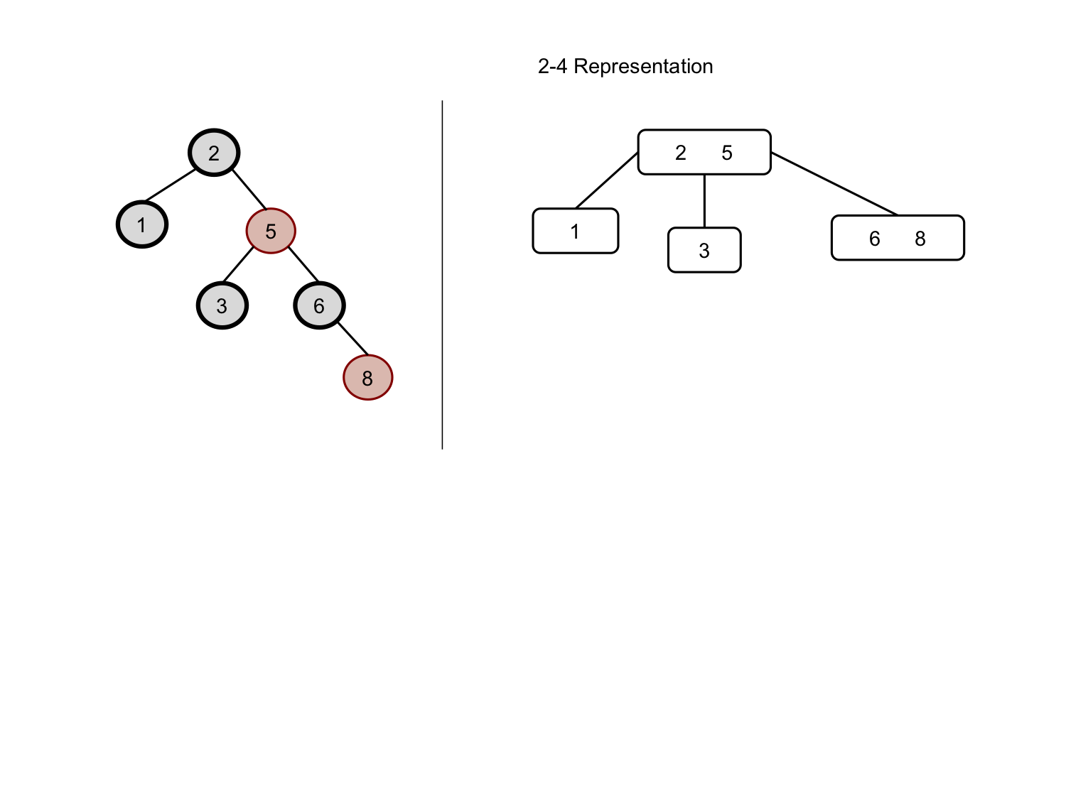
We will work through deleting the root node where key-value = 2…
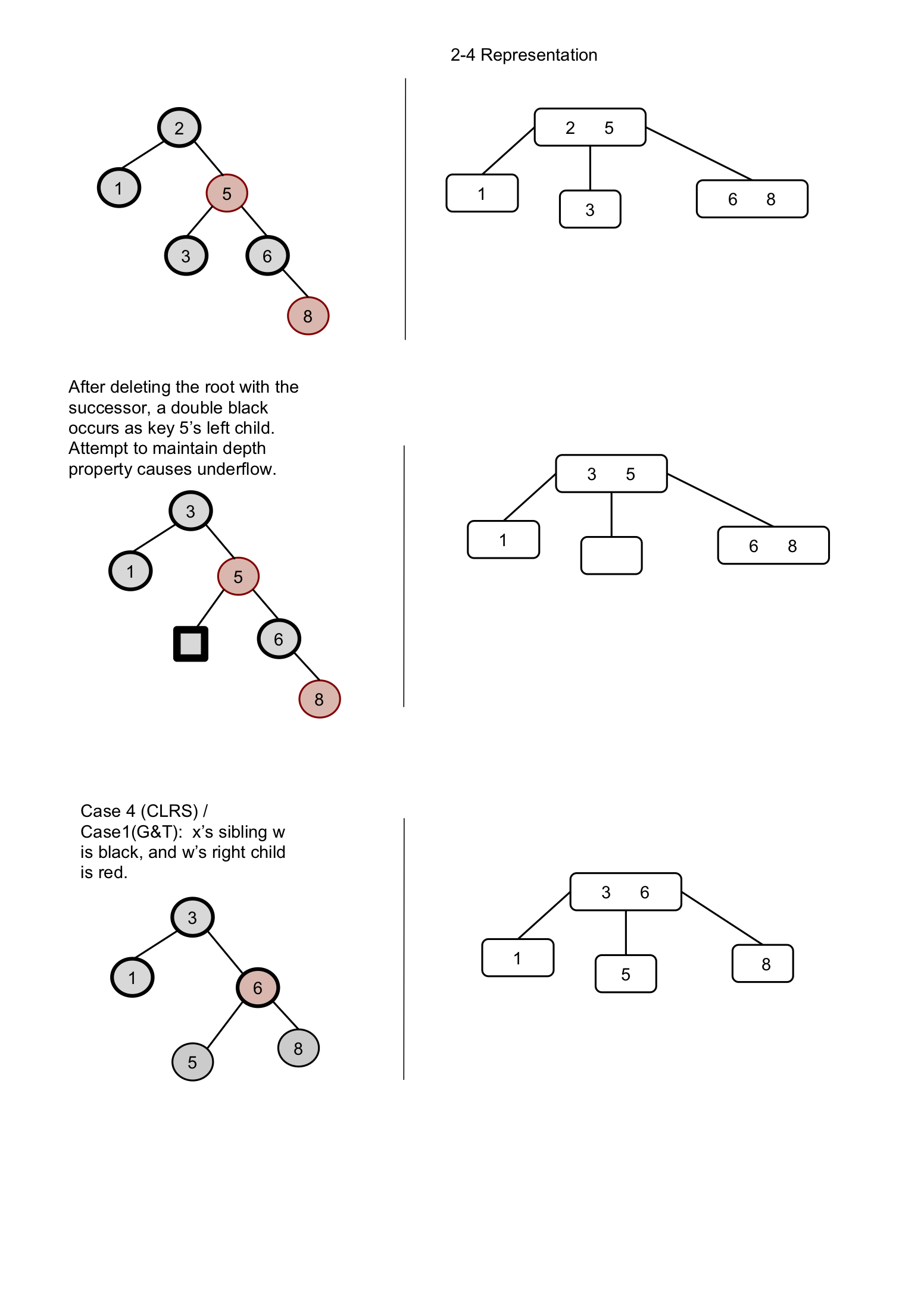
We will now delete the node with key-value = 1…
Height of a Red Black Tree
Let’s determine the largest number of internal nodes possible on a red black tree of black height k, as well as the smallest. Also, what the corresponding 2-4 tree heights would be.
A path from the root to leaf can have at most one red node between every black node, so twice the number of black nodes plus the bottommost red node…
h = 2k + 1
A complete tree would maximize the internal nodes as…
n = 2h - 1
= 22k + 1 - 1
For a complete red black tree, the 2-4 hieght is simply the black height as every node is absorbed by the black parent..
2-4 height = k
The least number of internal nodes occurs when the tree is black as a raven’s feather…
k + 1 = lg ( n + 1 )
2k + 1 = n + 1
n = 2k + 1 - 1
Again the 2-4 height = k
Will the tree ever be black as a raven’s feather with the CLRS implementation? Let us see…
Claim:
if n > 1, the tree has at least one red node.
Proof:
If a node z is inserted and ends up at the bottom of the tree it is colored red in line 16, Insert_Fix-up is called regardless. In all cases, 1, 2 & 3, if the black depth or root properties are violated, node colors must be changed. z remains red, but the ancestors of z undergo color manipulation. Ensuring that if n > 1, then one node must certainly be red after insert, that particular node being z itself.
QED
Problem set 07
Dynamic Programming
We now enter the wonderful world of graphs! In this set we will be focusing on the exciting concepts of dynamic programming!
Longest Paths
To start off we will write code in javascript for the longest path through a graph that stores both the value and the path. We will then write a function to print the path…
/* Assume all values in next are initialized to 1 by the caller */

function Longest_Path_Memoized (G, u, t, dist, next) {
  if (u === t) {
    dist[u] = 0
    next[u] = u
    return (dist, next)
  }

  if (dist[u] > -infinity) {
    return (dist[u], next[u])
  } else {
    G.adj[u].forEach(function (v) {
      let alt = w(u, v) + Longest_Path_Memoized (G, v, t, dist, next)
      if (dist[u] < alt) {
        dist[u] = alt
        next[u] = v
      }
    })
    return (dist[u], next[u])
  }

  function Print_Longest_Path (u, t, next) {
    let temp = u
    print(temp)
    while (temp !== t) {
      print('-> ' + next[temp])
      temp = next[temp]
    }
  }
}
Analysis
All entries of next and dist must be initialized, so this affects the run time of Longest_Path_Memoized by O( V ). Each sub-problem represented by a node is solved once due to memoization. Therefore the dominating cost of the algorithm exists in the forEach loop comparing adjacent edges of each node along the longest path, or O( E ). The printing routine has to, in the worst case, iterate over an array that contains all of the nodes in the graph G. Thus the combined run-time of both algorithms is…
O( E + V + V )
= O( E + 2V )
= O( E + V )
Activity Scheduling
When scheduling activities, the greedy approach of taking the earliest compatible finish time works absolutely fine when maximizing the number of elements in a sequence of activities. The locally optimized choice corresponds to global optimization as well. In this problem, we look at activity revenue optimization which causes the greedy approach to break down. First, we’ll describe the optimal substructure of the problem, a mathematical recurrence relation, and finally implement the solution using dynamic programming.
Optimal Substructure
The optimal solution Aij must also include the optimal solitions to two problems for Sik and Skj. If there existed some other set A’ik of mutually compatible activities in Sik where the value of A’ik was greater than that of Aik, then we would use A’ik instead of Aik as an optimal solution to a sub-problem of Sij. This contradicts the assumption that Aij is an optimal solution. Similarly for Skj.
Recurrence
A recurrence relation can be defined by the following…

Below is pythonic pseudocode implementing our dynamic approach…
def Activity_Revenue_Optimizer (n, s, f, v):
  val = [0 ... n + 1, 0 ... n + 1]
  activity = [0 ...  n + 1, 0 ... n + 1]

  for i in range(0, n):
    val[i, i] = 0
    val[i, i + 1] = 0
  val[n + 1, n + 1] = 0

  for i in range(2, n + 1):
    for j in range(0, n - i + 1):
      k = j + i
      val[j, k] = 0
      l = k - 1
      while (f[j] < f[l]):
        if (f[j] <= s[l] and f[l] <= s[k] and
            val[j, l] + val[l, k] + v[l] > val[j, k]):
              val[j, k] = val[j, l] + val[l, k] + v[l]
              activity[j, k] = l
        l -= 1
  return (val, activity)
It would be useful to see a print out of the activities…
def Print_Activities (val, activity, i, j):
  if (val[i, j] > 0):
    k = activity[i, j]
    print(k)
    Print_Activities (val, activity, i, k)
    Print_Activities (val, activity, k + 1, j)
Analysis
Activity_Revenue_Optimizer requires O( n 3 ) time to compare some element to every other element in a two-dimensional array.
Print_Activities is, in the worst case, O( n ) if all activities are compatible and thus require printing.

Wyatt Hoodes
Pressured != crushed; Perplexed != despair